Adam Karvonen*, Can Rager*, Johnny Lin*, Curt Tigges*, Joseph Bloom*, David Chanin, Yeu-Tong Lau, Eoin Farrell, Arthur Conmy, Callum McDougall, Kola Ayonrinde, Matthew Wearden, Samuel Marks, Neel Nanda *equal contribution
This blog post was originally published with the SAE Bench beta release on December 10, 2024. We are now releasing SAE Bench 1.0. We’ve made substantial improvements, added new SAE architectures, and conducted further evaluations that qualitatively alter some of our earlier findings—these key updates are summarized below. For up to date and comprehensive details, please refer to the SAE Bench paper (https://arxiv.org/abs/2503.09532). For comparability, we leave our initial blogpost from December 2024 below. Neuronpedia's SAEBench Evaluation browser features both the new results (SAEBench – Jan 25) and previous results (SAEBench – Dec 24) as separate releases.
We made minor changes to the training code for ReLU SAEs, added Matryoshka SAEs, and standardized the training hyperparameters across SAEs. The new suite of SAEBench SAEs includes 7 variants:
Trained across 3 widths (4k, 16k, and 65k), 6 sparsities (~20 to ~640), on layer 8 of Pythia-160M and layer 12 of Gemma-2-2B. Additionally, we have checkpoints throughout training for TopK and ReLU variants for Gemma-2-2B 16k and 65k widths. The SAEs are located in the following HuggingFace repos:
Find the evaluation results in the SAEBench interface by selecting the SAEBench - Jan 25 release.
In the typically used L0 range of 20-200, Matryoshka SAEs perform best on the TPP, SCR, RAVEL, and Feature Absorption metrics, and near best on the Sparse Probing metric. However, Matryoshkas do slightly underperform on the traditional sparsity - fidelity tradeoff. These differences are most apparent at the largest scale of 65k width, and improvements may be diminished or non-existent at smaller scales.
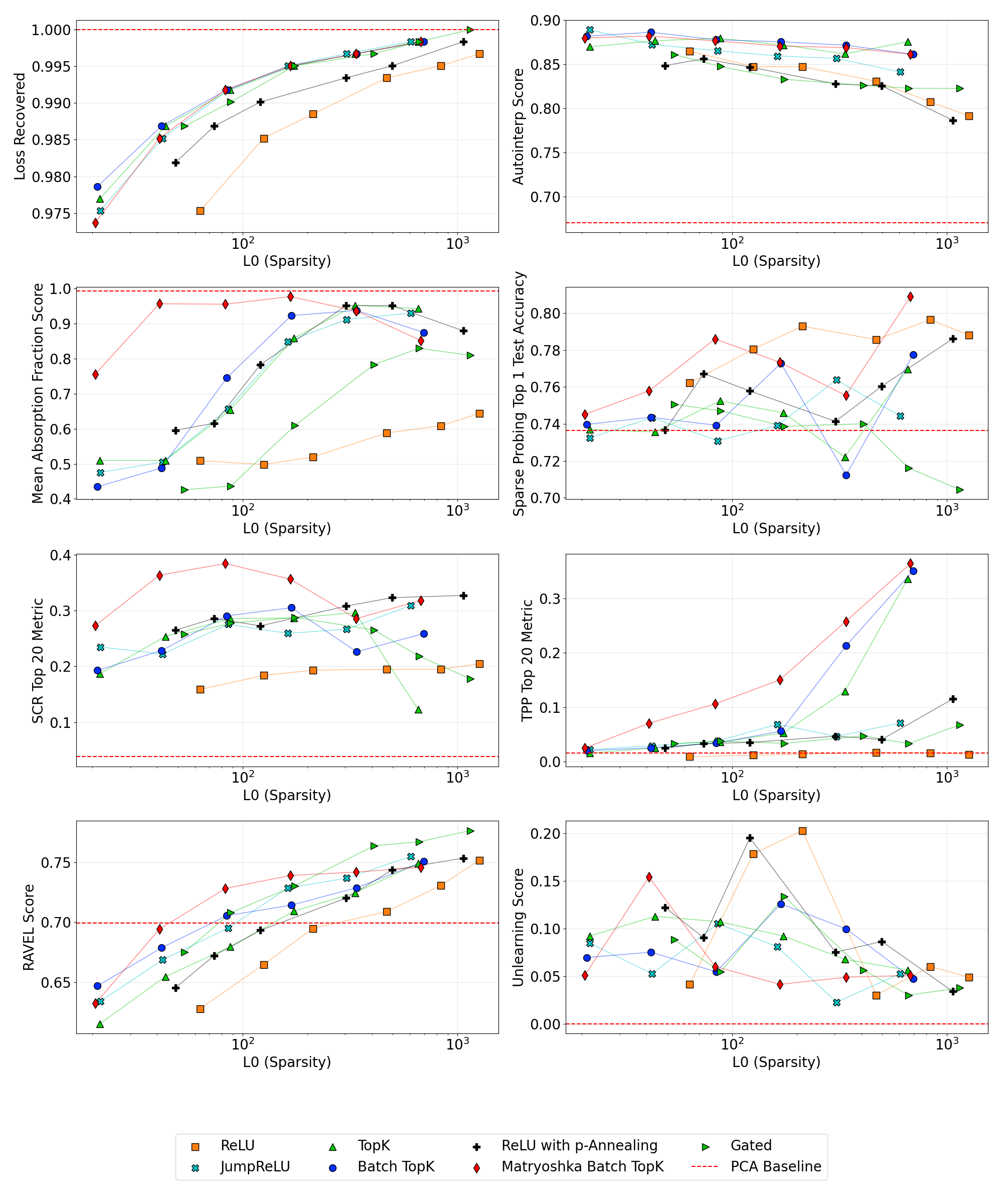 Scores for the Loss Recovered, Automated Interpretability, Absorption, SCR, and Sparse Probing metrics on the 65k width Gemma-2-2B suite of SAEs.
We also evaluated several proposed SAE approaches (TopK, BatchTopK, P-Anneal, Gated, JumpReLU) that had primarily focused on improving reconstruction accuracy. We observed it is often difficult to differentiate these approaches on our SAE Bench metrics. These findings emphasize the need for diverse metrics beyond proxies such as reconstruction accuracy.
Previously we had observed that there is no size / sparsity combination that appears to balance performance on all metrics. The SCR and Feature Absorption metrics had worse performance with scale, also called inverse scaling, for all previously tested SAE architectures. However, Matryoshka SAEs do not appear to have these trade-offs, and generally improve or maintain performance with increasing scale. A large Matryoshka SAE with an L0 of 50-150 may offer strong performance across a range of tasks, and we would be excited to see further investigation into the usage of Matryoshka SAEs.
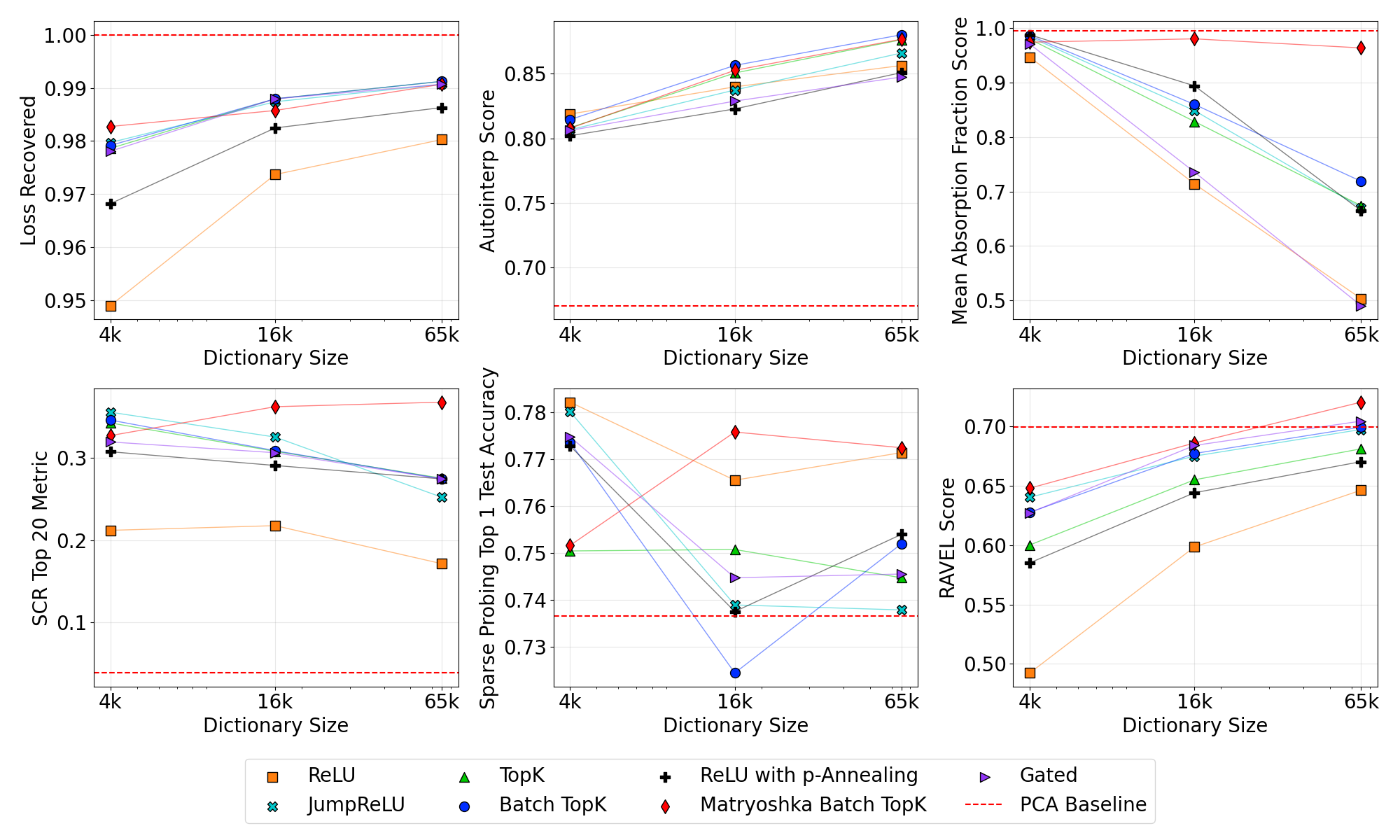 Scaling SAE width from 4k to 65k for across SAE architectures. For each architecture / width pair, we mean over all results in the L0 range between 40 and 200. Most notably the hierarchical Matryoshka SAE shows positive scaling behavior. Due to varying L0 distributions across architectures, this visualization is intended primarily for analyzing scaling
trends rather than architecture comparisons.
Scaling SAE width from 4k to 65k for across SAE architectures. For each architecture / width pair, we mean over all results in the L0 range between 40 and 200. Most notably the hierarchical Matryoshka SAE shows positive scaling behavior. Due to varying L0 distributions across architectures, this visualization is intended primarily for analyzing scaling
trends rather than architecture comparisons.
In our original blog post, we had found that ReLU SAEs had decreased levels of feature absorption. When training our baseline suite of SAEs, we improved our ReLU training approach from the original Towards Monosemanticity approach to the Anthropic April Update approach. After this improvement, we found that ReLU SAEs actually had the highest levels of feature absorption. After some inspection, we believe that the decreased feature absorption in our original results was due to a high percentage of dead features.
If an SAE effectively captures independent concepts, each should be encoded by dedicated latents, achieving clear disentanglement. To measure this, we implement the RAVEL (Resolving Attribute–Value Entanglements in Language Models) evaluation from Huang et al which tests how cleanly interpretability methods separate related attributes within language models. We’re excited to add this metric as it directly evaluates causal effects on downstream behavior. We find that RAVEL scores generally increase with L0, and for width 65k sparsity values between 40-200, Matryoshka performs best.
RAVEL evaluates whether targeted interventions on SAE latents can selectively change a model’s predictions for specific attributes without unintended side effects—for instance, making the model believe Paris is in Japan while preserving the knowledge that the language spoken remains French. Concretely, RAVEL works as follows: given prompts like "Paris is in the country of France," "People in Paris speak the language French" and "Tokyo is a city” we encode the tokens Paris and Tokyo using the SAE. We train a binary mask to transfer latent values from Tokyo to Paris, decode the modified latents, and insert them back into the residual stream for the model to generate completions. The final disentanglement score averages two metrics: the Cause Metric, measuring successful attribute changes due to the intervention, and the Isolation Metric, verifying minimal interference with other attributes.
Inspired by Heap et al, we evaluated SAEs trained on randomly initialized models as a baseline. We find that SAEs on trained models generally obtain significantly higher scores on our metrics, except for TPP. However, we caution that most of our metrics are meant for comparisons of different SAEs on the same model, and results should be interpreted with caution. For example, the TPP metric measures relative changes in probe accuracy within a given model. Given that the linear probes on the randomly initialized model start from a substantially lower baseline accuracy, direct comparisons of TPP across models may be misleading.
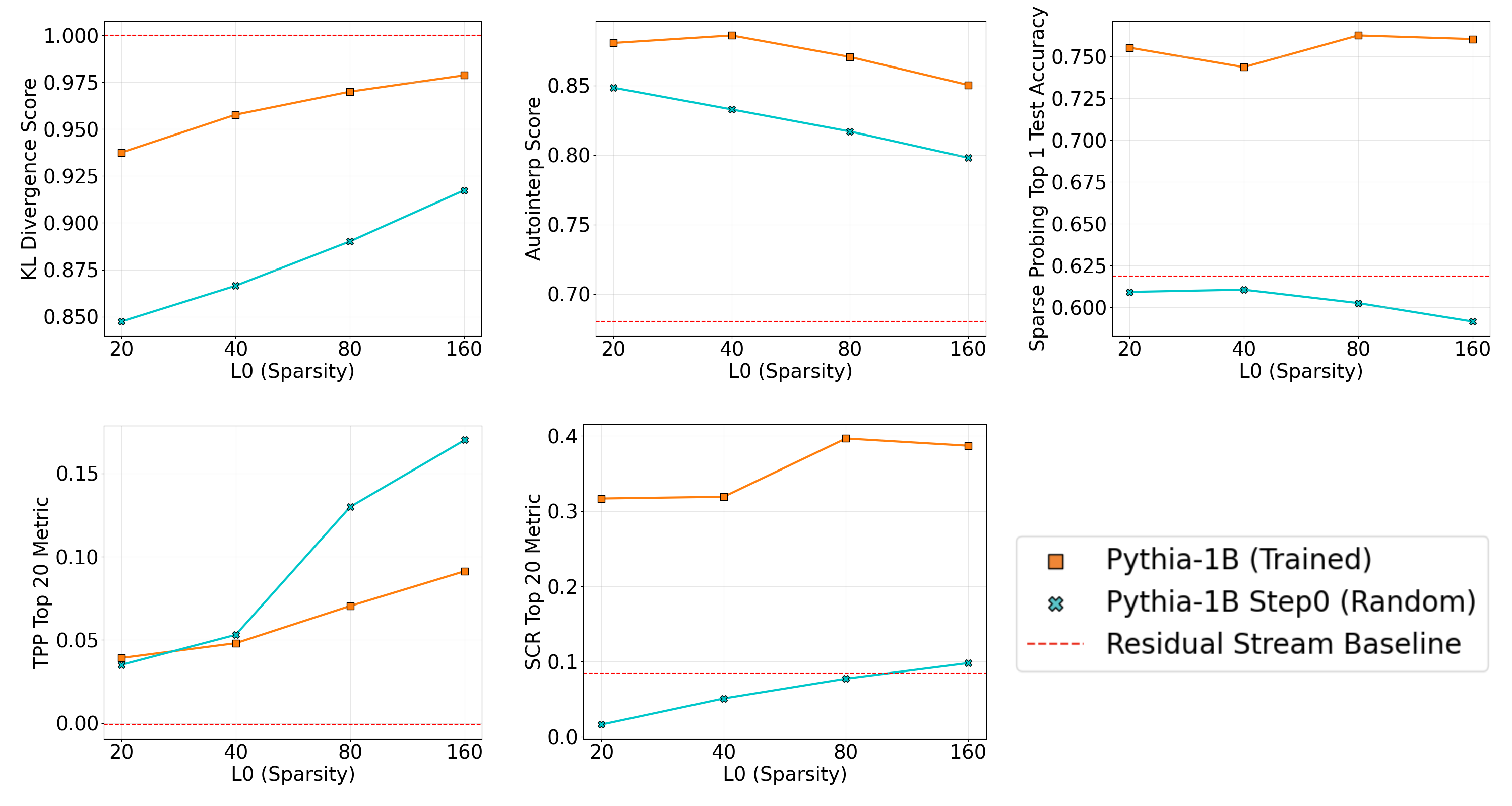 Evaluation results for SAEs trained on the randomly initialized and final versions of Pythia-1B.
Sparse Autoencoders (SAEs) have become one of the most popular tools for AI interpretability. A lot of recent interpretability work has been focused on studying SAEs, in particular on improving SAEs, e.g. the Gated SAE, TopK SAE, BatchTopK SAE, ProLu SAE, Jump Relu SAE, Layer Group SAE, Feature Choice SAE, Feature Aligned SAE, and Switch SAE. But how well do any of these improvements actually work?
The core challenge is that we don't know how to measure how good an SAE is. The fundamental premise of SAEs is a useful interpretability tool that unpacks concepts from model activations. The lack of ground truth labels for model internal features led the field to measure and optimize the proxy of sparsity instead. This objective successfully provided interpretable SAE latents. But sparsity has known problems as a proxy, such as feature absorption and composition of independent features. Yet, most SAE improvement work merely measures whether reconstruction is improved at a given sparsity, potentially missing problems like uninterpretable high frequency latents, or increased composition.
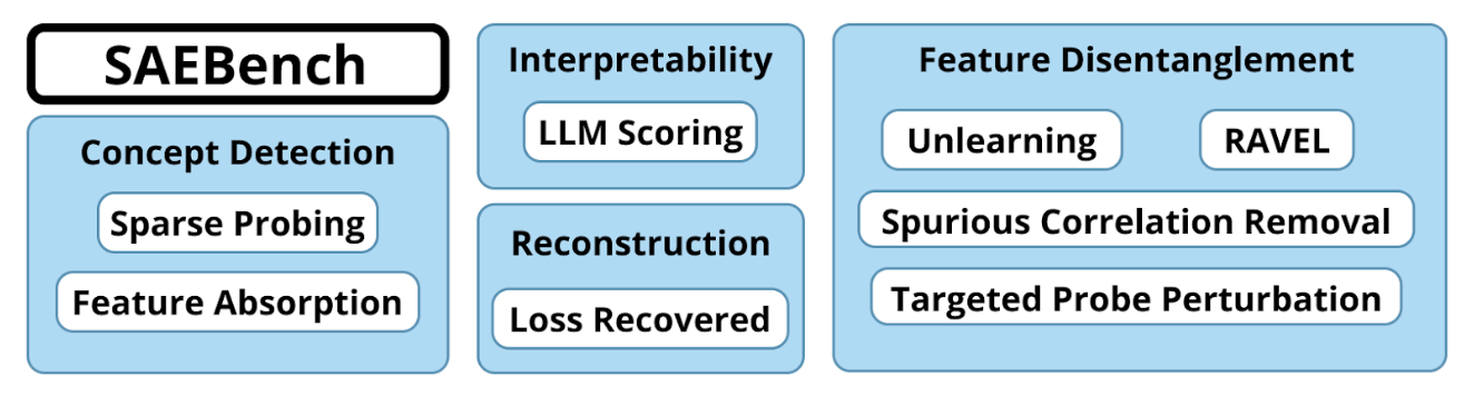
In the absence of a single, ideal metric, we argue that the best way to measure SAE quality is to give a more detailed picture with a range of diverse metrics. In particular, SAEs should be evaluated according to their performance on downstream tasks, a robust signal of usefulness.
Our comprehensive benchmark provides insight to fundamental questions about SAEs, like what the ideal sparsity,training time, and other hyperparameters. To showcase this, we've trained a custom suite of 200+ SAEs of varying dictionary size, sparsity, training time, and architecture (holding all else constant). Browse the evaluation results covering Pythia-70m and Gemma-2-2B on Neuronpedia.
SAEBench enables a range of use cases, such as measuring progress with new SAE architectures, revealing unintended SAE behavior, tuning training hyperparameters, and selecting the best SAE for a particular task. We find that these evaluation results are nuanced and there is no one ideal SAE configuration - instead, the best SAE varies depending on the specifics of the downstream task. Because of this, we cannot combine the results into a single number without obscuring tradeoffs. Instead, we provide a range of quantitative metrics so that researchers can measure the nuanced effects of experimental changes.
We are releasing a beta version of SAEBench, including a convenient demonstration notebook that evaluates custom SAEs on multiple benchmarks and plots the results. Our flexible codebase allows you to easily add your own evaluations.
What makes a good SAE? We evaluate several desirable properties with dedicated metrics.
Unfold the metrics below for detailed descriptions.
We provide implementations to measure sparsity and reconstruction error, the most commonly used metrics for comparing SAEs. We measure both the reconstruction error for the model's activations (Mean Squared Error aka MSE, fraction of variance explained, cosine similarity) and for the model's output logits (KL divergence, and change in cross-entropy loss). We also provide a range of unsupervised metrics, including feature density statistics, the L1 sparsity, and measures of shrinkage such as the L2 ratio and relative reconstruction bias.
| Metric | Description |
|---|---|
| L0 Sparsity |
|
| Cross Entropy Loss Score |
|
| Feature Density Statistics |
|
| L2 Ratio |
|
| Explained Variance |
|
| KL Divergence |
|
Sparsity incentivizes an undesirable phenomenon called feature absorption. Imagine an SAE learned two distinct latents tracking the features "starts with S" and "short". Since "short" always starts with S, the SAE can increase sparsity by absorbing the "starts with S" feature into the "short" latent and then no longer needs to fire the "starts with S" latent when the token "short" is present, as it already includes the "starts with S" feature direction.
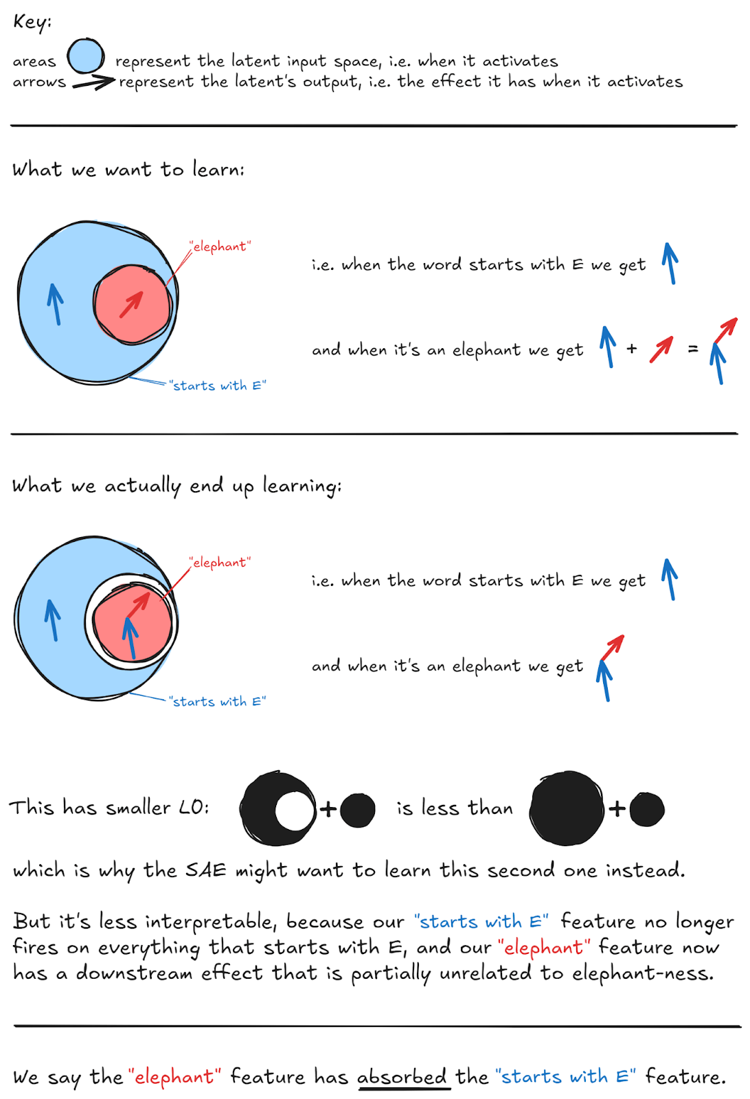
Credit: Callum McDougall, ARENA Tutorials
In general, feature absorption is incentivised any time there's a pair of concepts, A & B, where A implies B (i.e. if A activates then B will always also be active, but not necessarily the other way round). This will happen with categories/hierarchies, e.g. India => Asia, pig => mammal, red => color, etc. If the SAE learns a latent for A and a latent for B, then both will fire on inputs with A. But this is redundant–A implies B, so there's no need for the B latent to light up on A. And if the model learns a latent for A and a latent for "B except for A", then only one activates. This is sparser, but clearly less interpretable!
Feature absorption often happens in an unpredictable manner, resulting in unusual gerrymandered features. For example, the "starts with S" feature may fire on 95% of tokens beginning with S, yet fail to fire on an arbitrary 5% as the "starts with S" feature has been absorbed for this 5% of tokens. This is an undesirable property that we would like to minimize.
To quantify feature absorption, we follow the example in Chanin et al. and use a first letter classification task. First, tokens consisting of only English letters and an optional leading space are split into a train and test set, and a supervised logistic regression probe is trained on the train set using residual stream activations from the model. This probe is used as ground truth for the feature direction in the model. Next, k-sparse probing is performed on SAE latents from the train set to find which latents are most relevant for the task. The k=1 sparse probing latent is considered as a main SAE latent for the first letter task. To account for feature splitting, as k is increased from k=n to k=n+1, if the F1 score for the k=n+1 sparse probe represents an increase of more than τ_{fs} than the F1 of the k=n probe, the k=n+1 feature is considered a feature split and is added to the set of main SAE latents performing the first letter task. We use τ_fs=0.03 in line with Chanin et al.
After the main feature split latents for the first letter task are found, we look for test set examples where the main feature split latents fail to correctly classify the token, but the logistic regression probe is able to correctly classify the sample. We then look for a different SAE latent that fires on this sample that has a cosine similarity with the probe of at least τ*{ps}, and where the SAE latent accounts for at least τ*{pa} portion of the probe projection in the activation. We use τ*{ps}=0.025 and τ*{pa}=0.4 in line with Chanin et al..
This probe projection criteria is different from the metric in Chanin et al., where a minimum latent ablation effect is used instead. However, latent ablation cannot work at later layers of the model after the model has moved first-letter information from the origin token to the prediction point, and thus limits the applicability of the metric. Using a probe direction contribution criteria allows us to apply this metric at all layers of the model and is thus more suitable for a benchmark.
We evaluate SAEs on their ability to selectively remove knowledge while maintaining model performance on unrelated tasks, following the methodology in Applying sparse autoencoders to unlearn knowledge in language models.
This SAE unlearning evaluation uses the WMDP-bio dataset, which contains multiple-choice questions containing dangerous biology knowledge. The intervention methodology involves clamping selected SAE feature activations to negative values whenever the features activate during inference. Feature selection utilizes a dual-dataset approach: calculating feature sparsity across a "forget" dataset (WMDP-bio corpus) and a "retain" dataset (WikiText). The selection and intervention process involves three key hyperparameters:
retain_threshold - maximum allowable sparsity on the retain setn_features - number of top features to selectmultiplier - magnitude of negative clampingThe procedure first discards features with retain set sparsity above retain_threshold, then selects the top n_features by forget set sparsity, and finally clamps their activations to negative multiplier when activated.
We quantify unlearning effectiveness through two metrics:
Both metrics only evaluate on questions that the base model answers correctly across all option permutations, to reduce noise from uncertain model knowledge. Lower WMDP-bio accuracy indicates successful unlearning, while higher MMLU accuracy demonstrates preserved general capabilities.
We sweep the three hyperparameters to obtain multiple evaluation results per SAE. To derive a single evaluation metric, we filter for results maintaining MMLU accuracy above 0.99 and select the minimum achieved WMDP-bio accuracy, thereby measuring optimal unlearning performance within acceptable side effect constraints.
In the SHIFT method, a human evaluator debiases a classifier by ablating SAE latents. We automate SHIFT and use it to measure whether an SAE has found separate latents for distinct concepts – the concept of gender, and the concepts for someone's profession for example. Distinct features will enable a more precise removal of spurious correlations, thereby effectively debiasing the classifier.
First, we filter datasets (Bias in Bios and Amazon Reviews) for two binary labels. For example, we select text samples of two professions (professor, nurse) and the gender labels (male, female) from the Bias in Bios dataset. We partition this dataset into a balanced set—containing all combinations of professor/nurse and male/female—and a biased set that only includes male+professor and female+nurse combinations. We then train a linear classifier C_b on the biased dataset. The linear classifier picks up on both signals, such as gender and profession.
During the evaluation, we attempt to debias the classifier C_b by selecting SAE latents related to one class (eg. gender) to increase classification accuracy for the other class (eg. profession).
We select set L containing the top n SAE latents according to their absolute probe attribution score with a probe trained specifically to predict the spurious signal (eg. gender). Karvonen et al. found that the scores obtained with feature selection through probe attribution had a strong correlation with scores obtained with feature selection using an LLM judge. Thus, we select features using probe attribution to avoid the cost and potential biases associated with an LLM judge.
For each original and spurious-feature-informed set L of selected features, we remove the spurious signal by defining a modified classifier C_m = C_b L where all selected unrelated yet with high attribution latents are zero-ablated. The accuracy with which the modified classifier C_m predicts the desired class when evaluated on the balanced dataset indicates SAE quality. A higher accuracy suggests that the SAE was more effective in isolating and removing the spurious correlation of e.g. gender, allowing the classifier to focus on the intended task of e.g. profession classification.
We consider a normalized evaluation score:
S_{SHIFT} = (A_{abl} - A_{base}) / (A_{oracle} - A_{base})where, A_{abl} is the probe accuracy after ablation, A_{base} is the baseline accuracy (spurious probe before ablation), and A_{oracle} is the skyline accuracy (probe trained directly on the desired concept).
This score represents the proportion of improvement achieved through ablation relative to the maximum possible improvement, allowing fair comparison across different classes and models.
SHIFT requires datasets with correlated labels. We generalize SHIFT to all multiclass NLP datasets by introducing the targeted probe perturbation (TPP) metric. At a high level, we aim to find sets of SAE latents that disentangle the dataset classes. Inspired by SHIFT, we train probes on the model activations and measure the effect of ablating sets of latents on the probe accuracy. Ablating a disentangled set of latents should only have an isolated causal effect on one class probe, while leaving other class probes unaffected.
We consider a dataset mapping text to exactly one of m concepts c in C. For each class with index i = 1, ..., m we select the set L_i of the most relevant SAE latents as described in section [ref]. Note that we select the top signed importance scores, as we are only interested in latents that actively contribute to the targeted class.
For each concept c_i, we partition the dataset into samples of the targeted concept and a random mix of all other labels.
We define the model with probe corresponding to concept c_j with j = 1, ..., m as a linear classifier C_j which is able to classify concept c_j with accuracy A_j. Further, C_{i,j} denotes a classifier for c_j where latents L_i are ablated. Then, we iteratively evaluate the accuracy A_{i,j} of all linear classifiers C_{i,j} on the dataset partitioned for the corresponding class c_j. The targeted probe perturbation score:
S_{TPP} = mean_{(i=j)} (A_{i,j} - A_j) - mean_{(i≠j)} (A_{i,j} - A_j)represents the effectiveness of causally isolating a single probe. Ablating a disentangled set of latents should only show a significant accuracy decrease if i = j, namely if the latents selected for class i are ablated in the classifier of the same class i, and remain constant if i
eq j.
In automated interpretability evaluation, we use gpt4o-mini as an LLM judge to quantify the interpretability of SAE features at scale in line with Bills et al.. Our implementation is similar to the detection score proposed by EleutherAI, the observability tool by Transluce is noteworthy as well. The evaluation consists of two phases: generation and scoring.
In the generation phase, we obtain SAE activation values on webtext sequences. We select sequences with the highest activation values (top-k) and sample additional sequences with probability proportional to their activation values. These sequences are formatted by highlighting activating tokens with <<token>> syntax, and prompt an LLM to generate explanations for each feature based on these formatted sequences.
The scoring phase begins by creating a test set containing top activation sequences, importance-weighted sequences, and random sequences from the remaining distribution. Given a feature explanation and the shuffled test set of unlabeled sequences, another LLM judge predicts which sequences would activate the feature. The automatic interpretability score reflects the accuracy of predicted activations.
If an SAE is working as intended, different concepts should have dedicated latents, i.e. they should be disentangled. RAVEL evaluates how well interpretability methods identify and separate facts in language models. For example, can we use the SAE to have the model think that Paris is in Japan but that the language is still French?
The dataset contains 5 entity types (cities, Nobel laureates, verbs, physical objects, and occupations), each with 400-800 instances and 4-6 distinct attributes. For example, cities have attributes like country, continent, and language. Attributes are tested using 30-90 prompt templates in natural language and JSON format, with both zero-shot and few-shot variants.
RAVEL evaluates feature disentanglement through a three-stage process:
For an entity E (e.g., "Paris"), the cause score measures if intervening on feature F_A successfully changes the model's prediction of attribute A (e.g., country) from its original value A_E ("France") to a target value A_E' ("Japan"). The isolation score verifies that this intervention preserves predictions for all other attributes B (e.g., language) at their original values B_E ("French"). The final disentanglement score averages cause and isolation metrics across, with higher scores indicating better attribute separation. For instance, when changing Paris's country from France to Japan, a well-disentangled model would make this change while keeping the language attribute as French rather than incorrectly changing it to Japanese.
Follow-up work by Chaudhary & Geiger adapted the RAVEL benchmark to sparse autoencoders. While our implementation is closely related to the original RAVEL evaluation, a differential binary masking-based latent selection in line with Chaudhary & Geiger is forthcoming.
We evaluate our sparse autoencoders' ability to learn specified features through a series of targeted probing tasks across diverse domains, including language identification, profession classification, and sentiment analysis. For each task, we encode inputs through the SAE, apply mean pooling over non-padding tokens, and select the top-K latents using maximum mean difference. We train a logistic regression probe on the resulting representations and evaluate classification performance on held-out test data. Our evaluation spans 35 distinct binary classification tasks derived from five datasets.
Our probing evaluation encompasses five datasets spanning different domains and tasks:
| Dataset | Task Type | Description |
|---|---|---|
bias_in_bios | Profession Classification | Predicting professional roles from biographical text |
| Amazon Reviews | Product Classification & Sentiment | Dual tasks: category prediction and sentiment analysis |
| Europarl | Language Identification | Detecting document language |
| GitHub | Programming Language Classification | Identifying coding language from source code |
| AG News | Topic Categorization | Classifying news articles by subject |
To ensure consistent computational requirements across tasks, we sample 4,000 training and 1,000 test examples per binary classification task and truncate all inputs to 128 tokens. For GitHub data, we follow Gurnee et al. by excluding the first 150 characters (approximately 50 tokens) as a crude attempt to avoid license headers. We evaluated both mean pooling and max pooling across non-padding tokens, and used mean pooling as it obtained slightly higher accuracy. From each dataset, we select subsets containing up to five classes. Multiple subsets may be drawn from the same dataset to maintain positive ratios ≥0.2.
The Neuronpedia interface contains benchmark results for Gemma-Scope SAEs (JumpReLU architecture, 16k - 1M width, on Gemma-2-2B and -9B models) and the open-source SAEBench suite of sparse autoencoders (Standard (ReLU) and TopK architecture, 4k, 16k, 65k width for Gemma-2-2B).
In addition to SAEs, we provide the PCA of the residual stream (fit over a dataset of 200M model activations from the SAE training dataset) as a baseline. Note that the number of principal components is fixed to the model's hidden dimension (ie. hidden_dim = 2304 for Gemma-2-2B) while the number of SAE latents is often significantly higher.
Note that while we do compare Gemma Scope JumpReLU SAEs with our SAEs, the comparison is not apples to apples due to differences in training datasets, number of training tokens, training dataset context length, and other variables. We plan on training JumpReLU and Gated SAEs for direct comparisons of SAE architectures. In addition, we plan on investigating improvements to our Standard ReLU training approach, as our Standard SAEs currently have many dead latents.
Our feature absorption evaluation demonstrates the importance of having a suite of benchmarks to evaluate new methods. Optimizing the sparsity fidelity tradeoff, the field adopted JumpReLU and TopK sparse autoencoders which significantly worsened feature absorption. This is especially present at low L0 SAEs that are commonly used as they contain more human interpretable features. (Note, that feature absorption increases with training time. While the number of training tokens is comparable for Standard and TopK SAEs, the Gemma-Scope JumpReLU SAEs have been trained significantly longer.)
Absorption score across architectures for fixed 65k width. Note that unlike our other metrics, a lower score or rate of feature absorption is better.
Despite feature absorption, the new SAE architectures TopK and JumpReLU significantly outperform the standard ReLU architecture when evaluated on Layer 12 out of 26 in Gemma-2-2B. We therefore recommend the use of new architectures over Standard SAEs in line with Lindsey et al.
Diverse metric scores require tradeoffs in sparsity.
We find that metrics often vary across widths, sparsities, architectures, number of training tokens and model layers. Thus, we recommend to perform ablation studies when proposing new SAE architectures or evaluation metrics to ensure that the results are general and hold in a range of cases, rather than being an artifact of underlying variables such as sparsity. It is especially important to examine performance across multiple sparsities and model layers.
As examples, the impact of dictionary width on sparse probing varies significantly from layer 5 to layer 19 in Gemma-2-2B. In early layers, wider dictionaries are strictly worse, yet the results become more mixed in later layers. This may reflect how the model processes information, such as findings that later layers typically have more abstract features.
The optimum sparsity for sparse probing significantly varies between layers.
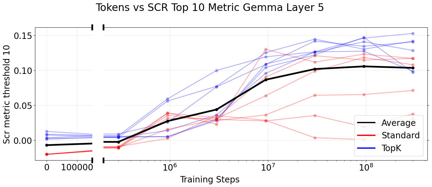
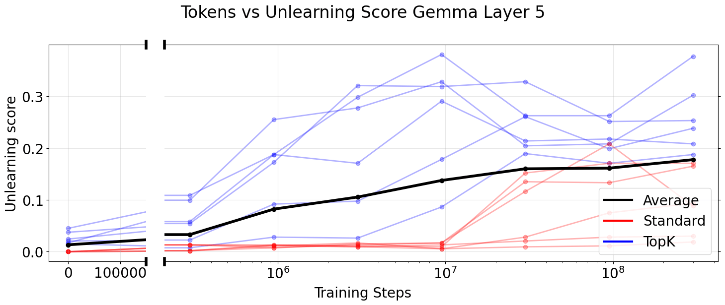
We further monitor performance on SAE Bench metrics throughout training and verify that metrics consistently increase on average. One initial motivation for the project was informing the duration of SAE training runs by signaling diminishing returns for performance on downstream applications. We observe that the number of training tokens before encountering a performance plateau significantly varies across metrics.
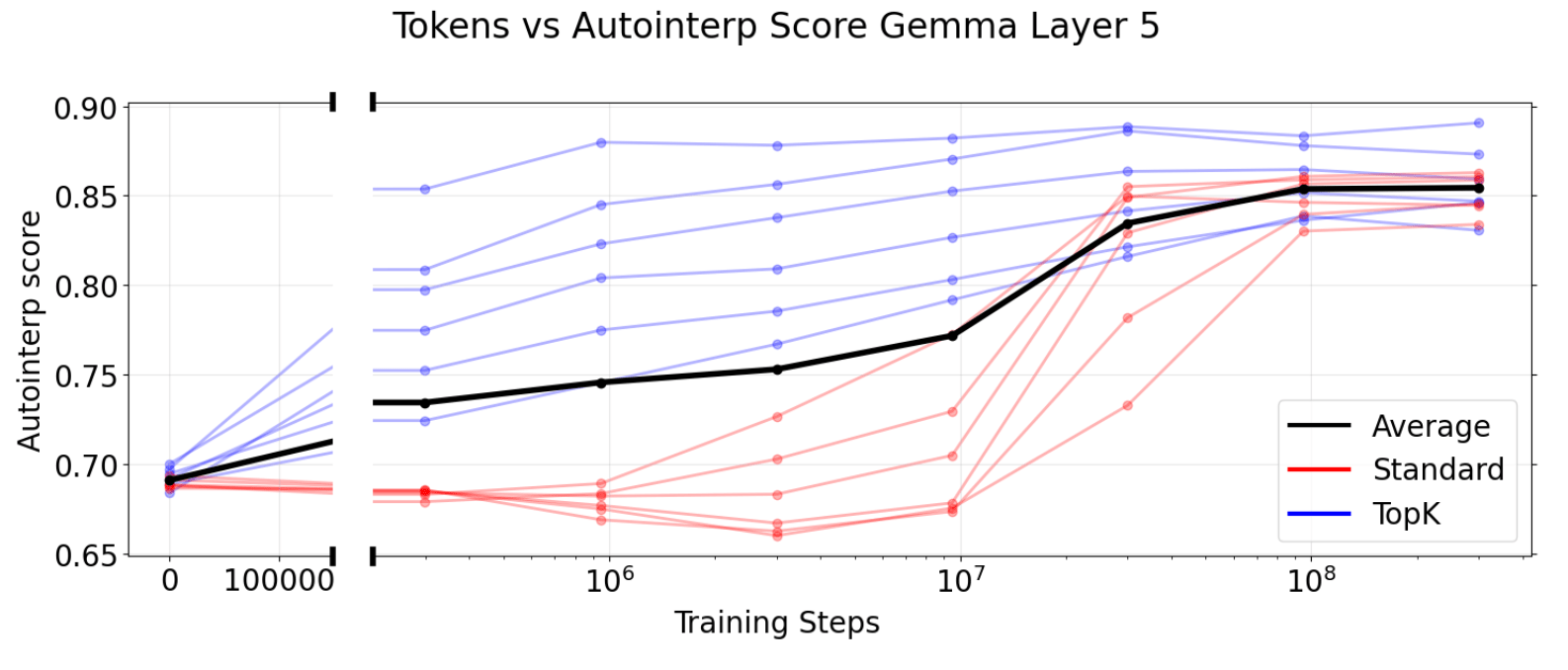
The automated interpretability score monotonically increases throughout training on average. Notably, TopK is more token efficient than the Standard SAE architecture.
One general application of SAEs is the controlled modification of model behavior1. For example, the debiasing technique SHIFT by Marks et al (CITE) modifies classification behavior through human selection of interpretable SAE latents. The number of features a human can manually select is limited, so we would prefer to make our modification using a smaller number of latents. In this case, smaller SAEs are clearly better for a fixed intervention budget in the lower L0 regime (left subplot). This is perhaps unsurprising, as with a fixed number of latents we are modifying a larger percentage of the smaller SAE.
The Spurious Correlation Removal (SCR) metric formulates SHIFT as an SAE evaluation. In the SCR setting, we automatically select SAE latents instead of relying on human judgement, effectively removing the intervention budget. Increasing the intervention budget from 10 up to 500 ablated latents, we do not see a clear advantage to using wider SAEs (right subplot).
![SAE Bench Gemma-2-2b TopK Width Series Layer 12 L0 vs SCR Best of [10,50,100,500]](/saebench/best-of.png)
The number of features per concept varies with (known as feature splitting). Given a concept removal task, the intervention budget therefore determines the optimal sparsity. In line with Sharkey, we observe that the choice of SAE width is a tradeoff between short description length and reconstruction error.
We also find that feature absorption gets worse with increased width.
For automated interpretability and reconstruction error however, we observe clear returns to increasing width.
The choice of optimal sparsity is highly dependent on the task as well. We clearly see the tradeoff between human interpretability and reconstruction loss.
SAEs in the high sparsity regime (low L0) perform relatively better on automated interpretability but worse on reconstruction error (Loss Recovered).
Even for similar downstream tasks we find different sparsities: Confusingly, unlike the closely related SCR evaluation, TPP has a strong correlation with sparsity, and higher L0 usually performs significantly better.
The optimal sparsity differs for SCR and TPP – two metrics that are conceptually closely related.
For some tasks lower L0 is typically clearly better, For other tasks, higher L0 is typically better. For other tasks such as SCR, there isn't a clear relationship with L0, but the best performance is generally obtained within a window of 20-200.
Better for Lower L0:
Non-Linear Relationship with L0:
Better for Higher L0:
We would love to hear your feedback. Get in touch with us via email.
This work was conducted as part of the ML Alignment & Theory Scholars (MATS) Program and supported by a grant from OpenPhilanthropy. The program's collaborative environment, bringing multiple researchers together in one location, made this diverse collaboration possible. We are grateful to Alex Makelov for discussions and implementations of sparse control, to McKenna Fitzgerald for her guidance and support throughout the program, as well as to Bart Bussmann, Patrick Leask, Javier Ferrando, Oscar Obeso, Stepan Shabalin, Arnab Sen Sharma and David Bau for their valuable input. Our thanks go to the entire MATS and Lighthaven staff.
@misc{karvonen2025saebench,
      title={SAEBench: A Comprehensive Benchmark for Sparse Autoencoders in Language Model Interpretability},
      author={Adam Karvonen and Can Rager and Johnny Lin and Curt Tigges and Joseph Bloom and David Chanin and Yeu-Tong Lau and Eoin Farrell and Callum McDougall and Kola Ayonrinde and Matthew Wearden and Arthur Conmy and Samuel Marks and Neel Nanda},
      year={2025},
      eprint={2503.09532},
      archivePrefix={arXiv},
      primaryClass={cs.LG},
      url={https://arxiv.org/abs/2503.09532},
}
Though SAEs surprisingly often work well, the choice of the most performant interpretability technique depends on the use case. ↩