Attribution Graphs for Studying Model Biology

Michael Hanna, Owen Lewis, Emmanuel Ameisen

Lindsey et al. described ten investigations of model behavior using attribution graphs and intervention experiments. These investigations surfaced a variety of interesting mechanisms in Claude 3.5 Haiku involved in behaviors like multi-step reasoning, planning, and hallucination inhibition.

Since then, the attribution graph method has been re-implemented by several groups. Participants in the Anthropic Fellows program released the Circuit Tracer library, which initially supported Gemma-2-2B and Llama-3.1-1B, and now Qwen3-4B as well. The initial release used per-layer transcoders (PLTs) (including Gemma transcoders trained by Gemma Scope), and more recently cross-layer transcoder (CLT) support has been added. Independently, EleutherAI released a separate attribution graph library (Attribute), which supports CLTs. Goodfire also implemented CLT-based attribution graphs internally, and used them to study the “greater than” circuits in GPT-2.

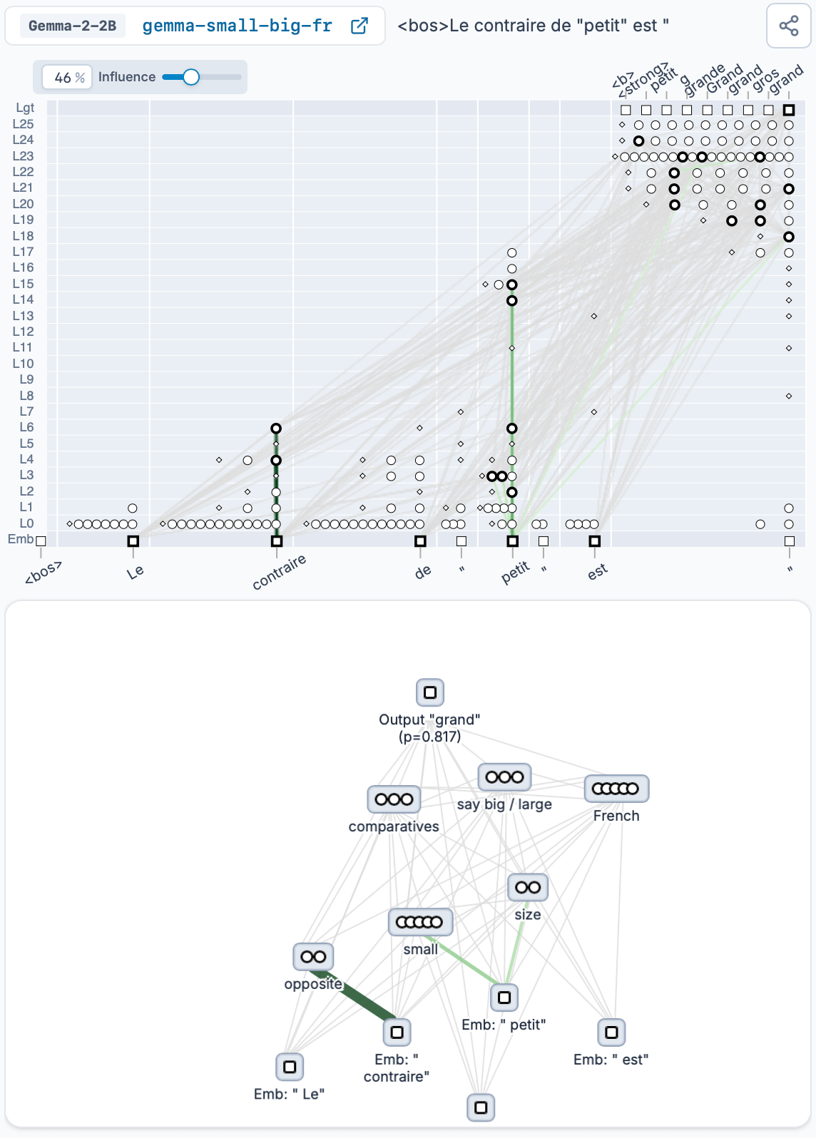
These replications have reproduced many of the findings of the original attribution graph paper. They surface generally sensible causal graphs which reveal both expected and unexpected mechanisms, with some uninterpretable components and missing pieces. As these methods have been applied to small models, the behaviors being studied and the corresponding mechanisms uncovered are often less “exciting” than those found on Haiku – extending these tools to larger models is ongoing work. Some examples of observations thus far include:

• Studying two-hop reasoning prompts on Gemma-2 (2B), a relatively weak model, showed that given inputs like “The state containing Dallas has its capital in”, Gemma-2 (2B) first activated “Texas” features, and then activated “Say Austin” features. Circuit tracing allows us to see that this intermediate hop was used, in addition to “shortcut” paths going straight from Dallas to Austin.

Gemma-2-2B graph for the prompt "The state containing Dallas has its capital in". [Open in Neuronpedia]

• Gemma-2 (2B) solves non-English reasoning tasks using a language-agnostic mechanism, and only later adds in language-specific features; language and task specific features can be intervened on independently. The existence of language-agnostic mechanisms and features was observed previously (Wendler et al.), however, the circuit connecting these mechanisms to language-specific features was not previously clear.

Gemma-2-2B graph for the prompt 'Le contraire de "petit" est "'. [Open in Neuronpedia]

• Llama-3.2 (1B) has features that track clause boundaries and uses them when processing ambiguous sentence fragments, as found by Hanna and Mueller. These features decide between readings of fragments like "Because the suspect changed the file", where it might be that the suspect is the subject ("Because the suspect changed the file, he was arrested") or the direct object ("Because the suspect changed the file was discarded"). Intervening on these features causes the model to change its continuation of the fragment. Transcoder circuits highlighted the existence of features representing “this token ends a clause” or “this token is a sentence’s subject."

• Models have features that track letter-level properties of individual tokens. This is especially (but not exclusively) the case in circumstances where the spelling or phonetics of the word are salient, such as acronyms and rhymes; for example, we see features that track qualities like “begins with the letter A”, or “contains the letter i.” Interestingly, however, these features often seem like imperfect match for the rhyme or wordform in question; to predict a word rhyming with “bent”, models appear to use features promoting words that “end in -nt”, “end in -en”, and “end in -es”, along with dedicated “*ent” rhyme features. It is not yet clear whether this reflects a genuine “consensus of heuristics” mechanism in the underlying model, or an artifact of feature splitting in the transcoder.

• Goodfire used CLTs to study the "greater-than" mechanism in GPT-2, following Hanna et al, inspecting an attribution graph for the prompt "The war lasted from the year 1711 to 17" and trying to deduce how the model knows to predict a number greater than 11. The authors found that CLTs extracted relevant structure “out of the box” by producing interpretable features that contribute to task performance using a variety of heuristics. Some features played an important role by upweighting appropriate outputs only in very particular input contexts – for instance, a feature that only activates when the input year ends in a number close to 11, suppresses numbers less than “11” and promotes larger numbers. Some other features appeared to promote larger number predictions regardless of the input, a better-than-chance but often-incorrect heuristic in this task. Interestingly, they also find features such as a parity detector, which promotes even outputs given odd inputs, a seemingly inappropriate heuristic for this task. The authors note that the view this provides of the computation is somewhat different than the one that was identified by Hanna et al., especially due to the narrow input selectivity of some of the features. This specificity is likely to be a consequence of how sparse transcoders are incentivized to represent computation; the authors note that studying a family of attribution graphs over many different inputs could reveal a more global view of the circuit.

Other investigations can be found in the circuit-tracer repository. Since the original publication, Circuit Tracer has been extended to support both PLTs and CLTs, enabling researchers to reproduce the full range of analyses from this work. To help the community get started, we're also releasing several pre-trained CLTs. We encourage readers to generate their own circuits, either using the library or directly on Neuronpedia, which does not require provisioning any infrastructure. To date, over 7,000 attribution graphs have been generated on Neuronpedia.

Recently, a few extensions and modifications to the original attribution graph framework have been proposed: one that accounts for attention computations and one that replaces transcoders with an alternative kind of MLP replacement layer. These methods are not yet reproduced on open-source models, but we hope to support them in the future and welcome community contributions!

Limitations

The case studies above demonstrate that transcoder-based attribution graphs can recapitulate some results found with other methods and surface new results, but also have significant limitations. Many limitations are described in the original paper; we focus on a few we have found particularly notable in our subsequent investigations.

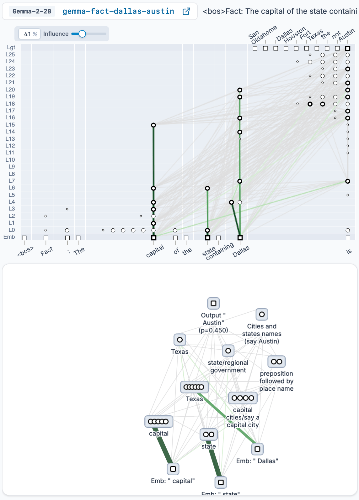
We have observed that transcoders can “shatter” geometric structures in the underlying model’s representation space. The objective functions used to train sparse replacement models encourage the preservation of information, but not the preservation of geometry. For example, Kantamneni et al. present evidence that Transformers use a helix-like number representation, and perform addition via trigonometric operations. However, attribution graph analyses of the same task don’t seem to recover this structure, but instead identify “lookup table features” corresponding to different possible combinations of inputs. Thus, while transcoders may match the prompt-for-prompt input/output behavior of a base model, they may not accurately reflect the global structure of representation spaces.

Relatedly, attribution graphs provide per-prompt analysis, using only a single example to discover mechanisms and show “what is going on in the model”. Thus, they represent “execution traces” rather than general algorithms. For example, they can show how the model computes 57 + 39, but not (directly) how it computes x + y, for universal x and y. Similarly, they can unwind the steps through which the model knows that Austin is that capital of the state containing Dallas, but can’t (directly) show how models store factual knowledge in general. Discoveries like the trigonometric structure of addition often emerge from studying many related prompts in aggregate, and distilling the computations and representations shared by all of them, resulting in an understanding of an algorithm as a whole. Future work could develop methods to automate this process by merging graphs from multiple prompts. Alternatively, new classes of replacement models could be trained to directly capture structured representation spaces that preserve the relationships between multiple inputs.

Finally, in many cases, error nodes are simply too prevalent in graphs and block us from tracing the important circuits.

Transcoder Architecture and Implementation

Stepan Shabalin*, Mateusz Piotrowski*, Curt Tigges*, Jack Merullo, Gonçalo Paulo

The original attribution graph papers (Ameisen et al., Lindsey et al.) used cross-layer transcoders (CLTs) as the basis of their attribution graphs, but noted that per-layer transcoders (PLTs) or even raw model neurons could also be used, with some tradeoff in sparsity, completeness, and/or interpretability. In this section we share some of our results from training CLTs and PLTs, and investigate some alternatives and extensions. We also document some important engineering considerations when training transcoders. Circuit Tracer now supports both CLTs and PLTs, enabling researchers to explore these tradeoffs directly.

Overall Findings

We tested a range of architectural variations on the basic CLT and PLT architectures on GPT-2 (for Llama 3.2 1B results, see Appendix B). We focused on the choice of activation function, the addition of skip connections, and weight-tying strategies. For circuit analysis, we ultimately want sparse attribution graphs that capture the most important computational pathways. We use replacement score as our measure of capturing computation.

We can modulate the replacement score / sparsity tradeoff in two ways: by varying the sparsity penalty during transcoder training, and by varying the aggressiveness with which we prune the resulting attribution graphs. Below we show the tradeoff for unpruned graphs, across a variety of architectures and activation functions.

We find that:

• CLTs generally outperform PLTs, even controlling for the number of parameters.

• JumpReLU, ReLU, and TopK are all reasonable choices for activation functions (using a Tanh sparsity penalty for the non-TopK options). JumpReLU performed the best for our CLTs, but requires more hyperparameter tuning, so TopK (or variants like BatchTopK) is a solid alternative.

• Skip PLTs, which in theory seemed like a promising way to capture cross-layer features at reduced computational cost, do not significantly outperform PLTs for GPT-2 (however, they appear to provide some advantage on Llama 3.1 1B – see Appendix B – though still not as much as CLTs.)

• Incremental ("weight-tied") CLTs that we tried do not outperform CLTs.

• Surprisingly, end-to-end finetuning does not improve replacement score despite reducing KL divergence of the “replacement model” given by the transcoders.

Training-time vs. Pruning-time Sparsity

The replacement scores and estimated L0 values in the chart above use unpruned circuit graphs. Typically, attribution graphs are pruned prior to analyzing them (see the pruning algorithm described by Ameisen et al.). Both training-time sparsity penalization and graph pruning are ways of achieving graph sparsity. To shed light on the different effects of these two ways of achieving sparsity, we took transcoders with the same architecture and varying unpruned sparsity levels, and pruned them with varying graph pruning thresholds. The following is for ReLU CLTs - see Appendix A for other architectures.

It can be seen that in order to target a final level of graph sparsity, using unpruned graphs is suboptimal, as is using too much pruning. Thus, practitioners should aim for transcoders to be less sparse than is ultimately desired, and achieve the rest of the sparsification via graph pruning. We estimate that to be roughly optimal, the training-time L0 should be chosen to “overshoot” the desired post-pruning sparsity by about 5–10×.

CLTs vs. PLTs

CLTs generally perform better in the sparsity regimes we are interested in (hundreds of active features per token, or less). JumpReLU CLTs performed best at the levels of sparsity we tested. However, we note that PLT performance, while worse, is not dramatically worse. For PLTs,  TopK and JumpReLU PLTs were similarly performant.

Activation Functions

Ameisen et al. used JumpReLU (Rajamanoharan et al.) as the activation function for training cross-layer transcoders, with a Tanh sparsity penalty. In addition to this setup, we explored TopK variants as well as classic ReLU.

We find that both JumpReLU and ReLU perform well, with a slight advantage for JumpReLU. However, both require careful hyperparameter tuning to achieve best performance. These parameters interact with each other in complex ways — while the sparsity penalty coefficient controls the L0, it's also impacted by the inner tanh coefficient parameter and learning rate. Getting these relationships wrong can result in large numbers of dead features (features that never activate) and poor performance. The preactivation loss from the original paper can help mitigate dead features, but it can also give a false illusion of improvement by keeping features alive that aren't contributing meaningfully to the computation.

TopK offers the advantage that we can directly set our target sparsity and doesn't require as much hyperparameter tuning. However, it also suffers from issues with learning many dead features, which can be counteracted with AuxK or preactivation loss.

When applying TopK to CLTs, we take the top K features from each layer. We also explored an alternative where we computed the “global” TopK across all layers simultaneously, which enables natural calibration of per-layer sparsities. An additional relaxation is BatchTopK, which sets average sparsity across the batch rather than per token, allowing varying numbers of active features per token while maintaining target average sparsity. We are still assessing the performance of these approaches, but early results are competitive with vanilla TopK on both training stability and final performance.

Skip Connections

Ameisen et al. found that CLTs are both more computationally expensive and more memory intensive than PLTs (given the same number of features), but lead to better replacement models even when computational cost is matched. Can the advantages of CLTs be captured at lower cost? Recently, other authors have explored “skip transcoders” (Paulo et al.) which augment transcoders with an additional (not-sparsity-penalized) linear connection. The use of skip-connections in PLTs improves their reconstruction loss, and could in principle capture some or all of the value of CLTs. A PLT endowed with skip connections induces an “effective CLT”, where a feature in layer L can be regarded as having “effective decoders” in layers beyond L, corresponding to their original decoder propagated through the skip connections at subsequent layers.

We find that Skip PLTs have lower reconstruction error than regular PLTs at the same level of sparsity, but this does not translate into better replacement scores. In general, we find skip variants underperforming their no-skip counterparts, with the exception of very high sparsity regimes. We believe skip connections may be transferring errors from previous layers, amplifying their impact on downstream computation. (Decoupling reconstruction error from replacement scores is possible because the replacement score calculations only give credit to the part of the linear skip term coming from previous layer features, while MSE calculations give credit to the entire linear skip term, including that coming from errors.) Thus, we don't consider skip PLTs to represent a clear improvement over standard PLTs, or a way to capture the benefit of CLTs.

Reconstruction Error and Replacement Score

We find that, while local reconstruction quality correlates with global circuit replacement scores, different architecture choices can create distinct trade-off patterns between these local and global metrics. As shown in the figure, there are distinct regimes corresponding to different architectural variants. In particular, adding skip connections results in lower replacement score at a given reconstruction error.

Incremental CLTs: A Weight-Tying Strategy

CLTs have significantly more parameters than PLTs, because for each layer there are as many decoders as layers “above” it. This increase in parameters makes training CLTs more memory intensive and therefore, more challenging for independent replications and local usage.

Incremental CLTs are a modification to CLTs that reduces memory usage by sharing weights that write to a particular layer. In a CLT, a feature with encoder in layer L writes to layers L+1, L+2, and so on. In an incremental CLT, a feature has an encoder and a decoder in every layer; the activity of the feature in layer L is the cumulative sum of the activity due to each encoder in that and previous layers.

Incremental CLTs can be implemented to use the same amount of FLOPs as PLTs with the same number of total features. We can compute the forward pass “incrementally” by cumulatively summing encoder contributions for features with tied decoders. This is a substantial FLOPs reduction compared to CLTs, if the CLTs are not implemented using sparse kernels. Note that the memory usage for activations will still increase because we cannot incrementally perform backward passes on each individual layer and free afterwards.

We found incremental CLTs to perform similarly to parameter-matched PLTs, but interestingly, incremental CLTs with a skip connection performed better (comparably to parameter-matched CLTs). We are still investigating the significance of these results.

We tried a different variant of weight-tied CLTs where decoder weights for the same feature are shared across layers. This variant has fewer parameters than CLTs but does not share the benefit of FLOP reduction. To make it work well, we needed to include learnable per-target-layer post-encoder offsets and scaling factors. Even after this modification, it did not outperform incremental CLTs on reconstruction error or replacement score.

KL Finetuning

Following Karvonen 2025, we tried to finetune transcoders on language modeling loss. To be precise, we compute KL divergence loss between a replacement model without error nodes (and all transcoders patched in at once) and the original model, then compute the sum of reconstruction error (variance-normalized MSE) losses over all layers, and then train on a sum of both with gradients normalized such that the value of the KL loss equals the summed NMSE loss (see paper mentioned above). The motivation is that this might push the reconstructions to preserve more of the computationally relevant structure and decrease the significance of error nodes in attribution graphs. We can successfully decrease KL divergence from 0.33 to 0.20 on a GPT2 skip-PLT after finetuning without significantly affecting the fraction of unexplained variance (0.226 → 0.23 on average). However, the replacement scores decreased with this change, from 0.723 to 0.705, so we did not pursue this further. It is possible we needed to put a higher weight on MSE loss to better preserve the original behavior, or that there is a better approach to end-to-end training than ours (e.g. end-to-end MSE loss). We leave a more thorough investigation to future work.

Implementation Considerations

• Storage and Shuffling

  • It's standard practice to shuffle data at the token level when training transcoders, but the storage requirements are massive—collecting 1B tokens from all layers of Llama-1B requires 130TB+ of storage. Full precaching is possible within cloud environments, but requires keeping both storage and GPUs in the cloud to avoid massive egress costs. For most researchers, the practical approach involves using smaller activation buffers with rolling shuffle buffers (1M+ tokens) that are refilled when depleted.

  • However, we find that even training without any shuffling has minimal impact on final model performance, though it makes training dynamics less stable. With sufficiently large batches, the benefits of shuffling may be less critical than commonly assumed.

• Training Monitoring For CLTs, we recommend tracking per-layer metrics separately, as different layers can exhibit very different training dynamics. For dead feature detection, instead of tracking the last active step, track the exponential moving average of activation density within batches. This provides more reliable dead latent detection and allows monitoring of density evolution throughout training, giving earlier warning of potential issues.

• Memory Management

  • CLTs present unique memory challenges since they require training all layers simultaneously, unlike PLTs where you can train subsets of layers independently. The dominant memory consumer is the decoder weight matrices, which scale quadratically with the number of layers—a feature in layer L needs decoders for layers L through the final layer.

  • We find that keeping model parameters in 16-bit precision maintains good performance, but Adam optimizer states must remain in fp32 with stochastic rounding enabled, otherwise training becomes unstable. Since Adam's optimizer states (particularly momentum terms) consume the majority of memory, this becomes the primary bottleneck. Gradient accumulation can help manage memory constraints, but be careful not to choose micro-batches that are too small, as this can hurt GPU utilization efficiency.

  • We've had some success training with Adam without momentum, which halves optimizer memory usage, but this approach is still under evaluation. We also found that in some cases we can keep the optimizer states in 8 bits (using torchao). Beyond tuning precision and optimizers, we suspect there may be significant redundancy in the decoder parameters themselves, suggesting potential optimization approaches for future work.

• Distributed Training

  • CLTs grow large quickly, so training reasonable sizes likely requires multiple GPUs. The standard approach is sharding along the feature dimension, requiring only one all-reduce operation for the final reconstruction. However, larger models quickly exceed single-node capacity (8 GPUs), and inadequate cross-host bandwidth can severely degrade training performance.

  • An alternative is sharding the decoder along the model dimension, combined with sparse activation functions. This replaces the all-reduce with an all-gather operation for feature activations, communicating only the indices and values of active features rather than dense reconstructions. This approach works with any sparse activation function, though TopK makes it particularly straightforward since the sparsity level is constant and predictable. Reducing memory requirements also helps with communication scaling, as smaller models can fit on fewer nodes with better interconnect bandwidth. (See Appendix G for distributed training implementation details.)

• Sparse Operations Because CLT features have decoders at many layers, the decoder step is much more FLOPS-intensive than the encoder step, creating substantial efficiency advantages for sparse operations. We compared several implementations and found Meta's PKM xformers embedding_bag kernels to be the fastest, but recommend torch.sparse in the CSR format for most uses because of its flexibility in representing varying sparsity levels. (See Appendix E and Appendix F for detailed FLOPS analysis and sparse kernel comparisons.)

Directions for Future Work

Neel Nanda, Jack Lindsey

In this section, we place attribution graphs and related circuit-tracing methods in context by considering next steps and possible directions for the field: opportunities for progress within this paradigm and by exploring alternative strategies altogether.

Alternative Strategies for Exploring Model Biology

There are many alternatives to hypothesis generation worth exploring besides attribution graphs, with different strengths and cost / performance tradeoffs.

• Training data attribution methods (e.g. influence functions) to find dataset examples responsible for a given output. Influence functions could also be applied to explain the dataset origin of feature activations or edges in an attribution graph.

• Scaling the process of reading a model’s chain of thought. How can we best analyze and aggregate them to look for unexpected properties, across many prompts? Docent is one interesting approach in this direction.

• Analyzing “token-space” mechanisms – for instance, approaches to identify causal relationships between aspects of the model’s sampled output (e.g. thought anchors)

• Linear probes can be highly effective at identifying concepts the model is representing – can we automate and scale the process of testing many linear probes, at all appropriate layers / token positions, for a given task?

• Simply observing model behavior in response to an appropriate mix of prompts can be highly effective to infer mechanistic hypotheses, but there’s an art to doing it well. What do best practices here look like? Can they be automated?

• Can we automate the full hypothesis generation + validation loop with LLM agents?

  • Automated hypothesis generation

    • Can LLMs simply guess the high-level casual graph of a task? Can an agent make more headway if we let it iteratively choose diverse prompts and read the output

    • How good are LLMs at interpreting an attribution graph and how good can we make them with the right prompt and scaffold?

  • Automated validation

    • Can we automate the design of probes to test for the presence of predicted features?

    • Can we automate intervention experiments, and synthetic / out-of-distribution inputs, used for hypothesis validation?

Open Questions About Key Model Mechanisms

• How do models perform “variable binding,” tracking and making use of information associated with a single entity?

• How do models aggregate information over long contexts? What state tracking algorithms are involved?

• Do models dynamically form in-context representations or circuits that have not been encountered before in the training data? Or does in-context learning recruit a preexisting repertoire of computational motifs?

• To what extent is factual or procedural knowledge stored “in one place” in the model, vs. being redundantly stored across multiple layers?

• What are the mechanisms underlying out-of-context learning?  In what sense are facts described in training documents internalized by the models?

• Under what circumstances do models form plans and take goal-directed actions? How rich can such plans be, and how are they represented?

• Do models have “meta-circuits” that select between different possible mechanisms?

• What kinds of information do models represent in a distributed fashion, “smeared” across many context positions?

Attribution Graphs

• Can we scale attribution graphs to long contexts – thousands or hundreds of thousands of tokens? What do such graphs look like  – are they dominated by a few token positions, or is computation spread out across many tokens?

• Can the process of analyzing an attribution graph – grouping together “supernodes,” identifying key pathways, validating circuits with perturbations – be made more systematic or even automated?

• Attribution graphs explain why a model behaved one way on a prompt, but not why it didn’t behave a different way.  How do we identify suppressive edges that were important to the model’s behavior?

• Attribution graphs give a “local” picture of model computation, specific to one prompt. Can we merge attribution graphs, or otherwise obtain a more global circuit picture?

• What can we learn for making attribution graphs that target quantities other than logit values – for instance, readouts of linear probes, or the activation of specific features?

• Recent work has extended attribution graphs to study attentional computations, and proposed several open questions for follow-up work.

Transcoders and Variants

• If we apply the idea of Matryoshka SAEs to (cross-layer) transcoders (CLTs), does it produce more interpretable features and graphs? Could we group hierarchically-related features in an automated fashion?

• Why are cross-layer connections helpful and what do they correspond to in the underlying model?

  • One hypothesis is that an MLP layer is partially explained by a linear component, and the cross-layer connections capture this linear propagation – however, if that’s the case, why do skip transcoders fail to perform as well when used for attribution graphs?

• Can we cut down the number of cross-layer connections in CLTs to reduce computational cost without compromising performance? For instance, by prioritizing cross-layer connections for features in certain layers, or allowing them only for a random subset of features, or restricting the layer range that a feature can write to.

• Can MLPs be decomposed into features at runtime without training a transcoder first? See e.g. Bushnaq et al. for an example of this approach, which identifies important directions in activation space by computing the singular value decomposition of Jacobians of model layers

• Can transcoders be circumvented altogether by training sparsity-regularized models from the start? See e.g. Park et al. for an example of this approach using a sparse mixture of experts model 

• What are the advantages and disadvantages of using sparse mixtures of linear transforms in lieu of transcoders?

Downstream Tasks

• Downstream tasks for measuring understanding: Much progress in machine learning has been driven by benchmarks, but benchmarks can also be misleading or only a proxy for what we actually care about in interpretability: understanding. What objectively verifiable, downstream tasks can we create that are directly about understanding?

  • Prior work includes Marks et al. and Cywinski et al. where model organisms with secret knowledge are created and audited to find these, and Movva et al. which tests the ability to generate natural language hypotheses that accurately explain a text dataset

  • Can we create an auditing games benchmark, where there are models with varying degrees of complex secret knowledge (from the simple hidden word in Cywinski et al to the rich and complex hidden goal in Marks et al) and we test the ability of our techniques to elicit it?

  • Can we teach our models hidden knowledge with fake fact finetuning, and see how well our techniques elicit it?

• How important is precision of mechanistic hypotheses? One notable consequence of the attribution graph approach vs, e.g. prompting, is that it can find much more nuanced and detailed hypotheses, like the addition analysis in Lindsey et al. For which kinds of downstream applications is this degree of precision important?

• Auditing games for model biology: Can we start to systematically measure the time taken from observing a novel model behaviour to finding a correct hypothesis for it (and validating that hypothesis) - how can we formalise and measure this, and compare the value of different tools for speeding up this process?

Biology of Chain-of-Thought / Reasoning Models

Models that use inference-time computation are increasingly important, but we understand very little about them – what can we learn about their biology? Between DeepSeek R1 and Qwen 3, there are multiple good open-weights reasoning models to study.

• How much can we trust the chain of thought (CoT)? Where is it insufficient to answer our questions about the model's true reasoning process? What methods can we design to flag misrepresentative CoT in an automated fashion / at scale?

• Can we tell the difference between a model deliberately rationalizing a preconceived answer in its CoT (as in the “implicit post-hoc rationalization” cases of Arcuschin et al., or the unfaithfulness example from Lindsey et al.) versus simply being mistaken in its reasoning?

• Can we tell when a CoT was causally important for a model giving its answer?

  • This is a subtle concept to pin down – models may have a causally irrelevant CoT that gives the same answer, and editing the CoT throws the model off distribution, which may change its answer for unrelated reasons.

• What factors lead to different forms of “unfaithful” CoT? Can we distinguish them?

  • Deliberately rationalizing a preconceived answer (Arcuschin et al., Lindsey et al.)

  • Models changing their answer because of a hint but not admitting it (Chen et al.)

  • Models taking logical shortcuts in maths problems after getting stuck, to claim they’ve achieved a valid “proof” (Arcuschin et al.)

  • Models giving a reasonable chain of thought, but at the last minute “flipping” to a different final answer (Arcuschin et al.)

Appendix

A. Additional Metrics

Post-pruning Replacement Scores for All Sparsity Sweeps

B. Llama 3.2 1B Results

We can see that the relationships between MSE, L0 and Replacement Score are similar between Llama 3.2 1B and GPT2:

• CLTs outperform PLTs.

• Normalized MSE and replacement score are highly correlated

• Skip transcoders reduce MSE for a given L0 level, but have worse replacement score at a given MSE

  • On Llama, they still provide an advantage on net.

• TopK, ReLU and Jump ReLU perform similarly.

C. Circuit Graph Construction Details

We compute replacement scores following pruning in the following way:

1. During pruning (prior to abs() + normalization): when a non-error node is removed, add its output contribution to the error node at the same layer index and position.

2. Compute the replacement score as usual – compute influence to error nodes and input embedding nodes and find the fraction of influence from input nodes.

D. Pseudocode for Incremental CLT

E. Sparse Kernels (EleutherAI)

For sparse transcoders, we are interested in computing a sparse-dense matrix multiplication. That is, on the left we have a very sparse vector of activations, and on the right we have a dense matrix with a large number of rows. For TopK SAEs, the sparse vector has shape (batch_size, k) where K is the K sparsity value. BatchTopK and JumpReLU SAEs can also use this format, but with some zero elements – we can pad their k to some multiple of the true value.

There are multiple implementations of this operation. OpenAI’s TopK SAE introduced several sparse matmul kernels that can be used to improve computational efficiency of SAE training and speed up all components of the backward pass that can be. Similar kernels have been implemented by Meta for their memory layer research. Torch also includes an implementation of CSR and COO sparse matmul.

We compared the forward passes from these implementations with torch.utils.benchmark on a sparse activation matrix with 2^20 rows and 2^19 columns (128 randomly selected elements active per row) and a dense decoder matrix with 2^19 rows and 2048 columns.

OpenAI and Meta’s kernels have similar performance. They are basically the same Triton kernel with some small differences. They work by loading rows of the decoder into shared memory, summing them and writing back to memory. We can estimate their performance by finding the number of decoder rows they need to load from VRAM, finding the size of each, and calculating the time it takes to load everything given the GPU’s memory bandwidth. In our tests, this is a very accurate approximation of their runtime, with the kernels achieving about 95% of the performance predicted by this bound. Dense matmul kernels can avoid the bandwidth bottleneck by reusing fetched decoder rows between activations, but this is likely impossible for sparse matmul.

torch.sparse.mm is only efficient in CSR format and has similar performance to OpenAI and Meta’s kernels. It is preferable over the latter because it has more flexibility in the number of columns per row thanks to the CSR format.

Keeping activations and the decoder in bfloat16 leads to a 2× speedup compared to float32. Having both or neither in bfloat16 is necessary for CSR.

All of these operations include backward passes:

OpenAI’s backward pass is simple, uses atomic operations and is the slowest. torch.sparse.mm slightly loses out to xformers_embedding_bag, which sorts indices before running a combined backward pass kernel.

The encoder backward pass requires the same set of operations as the decoder forward + backward pass. Xformers should theoretically be the best choice, but OpenAI’s kernels are easier to add in practice because the backward passes for all of the elements are separate and don’t require outside setup.

F. Sparse Kernels in JAX (DeepMind)

As part of our work on cross-layer transcoders, we’ve implemented a sparse version of the decoder matrix in a JAX-friendly way. The method is a slight modification of the core ideas in Gao et al’s work on sparse kernels.

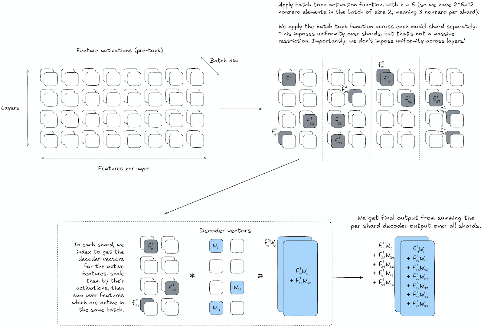
We perform only model parallelism during training (with model sharding happening along the feature dimension). Our activations array has the shape (batch_size, n_layers, features_per_layer). When we perform topk (or batch topk), we slice the activations only by their model sharding (i.e. into n_shards separate slices of size (batch_size, n_layers, features_per_layer // n_shards). For each shard, we perform the same operation: take the top k // (n_layers * n_shards) elements across the last dimension in the batch, where k is the target L0 across all layers of the model (or if we’re doing batch topk then we take the top k * batch_size // n_shards from the entire shard). This gives us the same number of activations in each shard, which we can then gather and return (kept in sparse form, i.e. just the nonzero values and their corresponding indices). These returned sparse activation arrays are still both sharded along the feature dimension (which is possible because of uniformity) but not sharded along the batch dimension (this is because for batch topk we have no way of imposing uniformity across elements in the batch). 

Now, the decoder weight has shape (n_layers_in, features_per_layer, n_layers_out, d_model), and is sharded along its second dimension (i.e. the features-per-layer dimension). We send each shard of the sparse input values & indices to its corresponding decoder slice, and perform a sparse matmul (i.e. indexing into the decoder matrix to extract the vectors corresponding to the nonzero activations, then summing over vectors corresponding to activations with the same batch index). This gives us activations of shape (batch_size, n_layers_out, d_model) for each shard, which we then sum together across shards to give us our final output.

Why is stacking activations by layer important? If we imposed shard uniformity across flattened activations of shape (batch_size, n_layers * features_per_layer), this would effectively mean that we had a uniform distribution of activations over layers in the model, which is definitely not what we want! CLT training (and even PLT training) should be free to distribute its activations over layers in a non-uniform way (and in fact, we’ve empirically observed that this does happen, with feature allocation per layer generally increasing throughout the model before a sharp drop-off in the final few layers). In contrast, imposing uniformity across the features_per_layer dimension is a much smaller constraint on the kind of solution that the model can learn (see next paragraph for a discussion of one possible constraint). It does provide some constraint: if two features are in different shards then they don’t suppress each other (i.e. one being active doesn’t prevent the other from also being active). We’re currently unsure whether this presents a significant enough cost to our CLTs to outweigh the performance gains at large scales - if it does, then we’ll instead adopt the alternative solution where topk isn’t taken over each shard separately, rather the whole batch of nonzero activations is sent to every shard, and we simply multiply these activations by a mask before using them to scale our decoder vectors (so we zero out all the activations which don’t correspond to this particular shard). This solution contains n_shards times more indexing into our decoder which is costly for JAX (since it’s a library optimized for matmuls not for indexing), however it’s the encoder forward pass and other operations still dominate the SAE training cost so this may end up not mattering much.

A note on the topk function - we use JAX’s approximate topk function rather than the fully accurate topk (because JAX handles operations like sorting less efficiently than matmuls). This function allows you to set a parameter recall_value (a float between 0 and 1), and it will return you a set of values & indices which have this overlap with the true topk values (in expectation). We haven’t finished experimenting with this parameter, but values between 0.7 and 0.95 have given good results. Note that as part of our investigations, we’ve discovered a mistake in the implementation of this function: specifically the formula (13) used in the original paper is based on an incorrect characterization of the problem. The result is that the parameter L is overestimated, and the resulting algorithm will give you a higher expected recall than your parameter (and will result in a function that takes slightly longer to run). This isn’t particularly important (especially if you’re using the regular topk function rather than batch topk, since the cost of the topk operation in this case is trivial), but worth mentioning.

Here is a diagram illustrating the batch topk algorithm, with uniform sharding across layers:

G. Distributed Training

A section of Appendix D.4 in Ameisen et al. is dedicated to distributed training and strategies for sharding parameters across accelerators. In that work, encoder and decoder is sharded with tensor parallelism, and accelerators are automatically allocated so that the fraction of memory used for parameters is constant. The encoder and decoder are sharded across the feature axis. Each accelerator computes its contribution to the output of the transcoder and an allreduce is made to sum across the feature axis.

A naive sharding implementation when training sparse coders is to shard across the layer axis with FSDP, but this approach soon finds problems with cross-layer transcoders because they require connections across layers.

EleutherAI's clt-training library implements a sharding optimization that is useful when not having access to a lot of GPUs. Instead of using an activation buffer, compute them on the fly. This doesn’t require an activation cache, and the gradients can be computed for a transcoder before the next layer’s activations are known. This means they can’t take advantage of shuffling, but in turn, can reduce memory usage and implementation complexity. It also means it is possible to easily finetune transcoders for KL divergence and other end-to-end losses without removing the cache.

In their implementation, the forward pass uses different data for each accelerator. While it is possible to shard model parameters across devices, at scales relevant for the open source community (1B-2B) there is not much point to doing this – model parameters and activations will take up a tiny fraction of GPU memory. After computing the input and target activations at a given MLP layer, they are all-gathered across the tensor parallelism axis to get the same set of tokens on each TP rank.

Once the sparse activations from the local encoder are available on each rank, they are reduced with an all-gather and run another top-K on gathered activations, similarly to Gao et al. After that, the decoder forward pass uses the aforementioned sparse kernels. Target activations (MLP outputs) as well as decoder weights are sharded across the model dimension, meaning the forward pass through the decoder, loss computation and the first part of the backward pass can be computed entirely locally on one TP rank. After the backward pass through the decoder, we allgather the sparse gradients on the GPUs. We then filter gradients belonging to each rank before performing a local sparse encoder backward pass.

Successfully implementing this strategy requires the use of sparse kernels, or at least sparsification as an intermediate step in the encoder forward pass. This is because the communication after the encoder is performed across the feature dimension and would be more expensive than a d_model communication if we needed to send dense post-activation latents.

If the implementation does not make activations sparse, we recommend the usual strategy of sharding both the encoder and decoder across the feature dimension. This way, the forward and backward passes are entirely local, with only one sum allreduce at the end. 

To benchmark this distributed implementation we ran evaluations with torch.utils.benchmark using 4 A40s in one node with 2^19 latents, a batch size of 2^16 and K=64, with all weights in bfloat16. By default, a forward+backward pass achieves 47.8% FLOPs utilization (as compared to the theoretical encoder forward pass + 3 equivalent backward sparse operations). With Xie et al.2025’s RTopK kernels for TopK, utilization becomes 53.8%. With sharding over the feature dimension instead of the output dimension, utilization for the combined forward+backward pass drops to 40%. With the Groupmax activation function instead of TopK, utilization is 65.3%.

We want to note that the strategy used by EleutherAI is not the most memory- or time- efficient option for managing activations – one could interleave computation and communication by running the encoder on the local batch while sending the current batch and previous activations over to the next TP processor in a ring, storing only computed and received sparse activations and concatenating them in the end. One would never need to store activations from all ranks at once, and memory would only be used for the negligibly small sparse activations. We could also likely mask the expensive d_model all-gather with the similarly expensive encoder forward pass. To our knowledge, there is currently no public implementation of this method, and altering EleutherAI/clt-training to allow for this optimization is unfortunately non-trivial.